Introduction
To build and inspect the interactions between the layers that make up an inference engineering stack, a system that naturally connects all the dots is Inferex. Inferex is a benchmark-driven LLM inference platform. The goal is to see what it takes to run an LLM effectively in a production setting, and to have the rigour of evaluating the major subsystems along the way: inference engines, the API gateway, quantisation pipelines, observability, and Kubernetes deployment.
The question every component had to answer before becoming a dependency was: Does this reflect how a production inference platform is actually built?. That question shaped every design decision and kept the scope from exploding.
There is no inference without hardware. The hardware capacity is one of the primary reasons LLMOps is tricky. It automatically determines how large you can go in Large
language models operations. GPU memory determines not only how large a model can be served, but also how much KV cache remains available for concurrent requests and long contexts. For inferex, a consumer Blackwell GPU, the RTX 5090 with 32 GB VRAM, running on WSL2, was used. The constraints introduced by that environment, and the workaround required to operate modern inference engines within it, became part of the investigation itself.

Implementation Scope
Inferex sits above inference engines rather than inside them. It does not implement attention kernels, schedulers, or memory managers. Those responsibilities belong to engine developers working on projects such as vLLM and SGLang.
Instead, Inferex focuses on the activities expected from an inference engineer:
- Selecting inference engines
- Configuring serving stacks
- Warming up engines
- Measuring behaviour under load
- Comparing engines fairly
- Observing performance metrics
- Operating engines within hardware constraints
- Producing evidence that informs engineering decisions
The article progresses layer by layer: from the gateway through the engines, quantisation benchmarks, observability, Docker and Kubernetes.
The Gateway
Suppose we deploy vllm serve llama3 to the public internet. It works for one user, or maybe ten. Eventually problems emerge. Authentication, Rate limiting, Logging, Metrics, Health checks, Streaming, and Observability. Then users arrive in hundreds and thousands. Some are legitimate while others are abusive. Some disconnect mid-stream while some send enormous prompts. To effectively handle these, a subsystem have to be responsible for managing all of these issues for efficient and fair access. That is the job of The Gateway.

The gateway serves as the control plane in order to protect the inference engine. It exists between the client and the engine to manage activities around:
- Authentication: Who is allowed to call this?
- Rate limiting: Control traffic i.e How much can one caller consume within a given time?
- Observability: What is actually happening?
- health Monitoring: Is the system alive?
- Secret management: How are credentials handled?

The four-layer control plane
Every request that enters inferex passes through four layers in sequence before it reaches inference engine. Each layer has one job. No layer knows about the others.
-
Layer 1: Authentication — X-API-Key, 401 vs 403
The first question the gateway asks is simple: who is this? Every request must carry an
X-API-Keyheader. If the header is absent, the gateway returns401(the caller did not identify themselves). If the header is present but the key is not in the configured set, the gateway returns403(the caller identified themselves, but they are not allowed in). The distinction matters.401means try again with credentials.403means your credentials are known and rejected. The key set lives in an environment variable,GATEWAY_API_KEYS, loaded at startup. No database. No round-trip. The check is a membership test against a set in memory — fast enough that it adds no measurable latency to the request path.#Authentication dependency snippet async def require_api_key( x_api_key: Optional[str] = Header(default=None, alias="X-API-Key"), ) -> str: """Validate the X-API-Key header; raise 401 if absent, 403 if unrecognised.""" if x_api_key is None: raise HTTPException( status_code=status.HTTP_401_UNAUTHORIZED, detail="Missing X-API-Key header", headers={"WWW-Authenticate": "ApiKey"}, ) if x_api_key not in VALID_API_KEYS: raise HTTPException( status_code=status.HTTP_403_FORBIDDEN, detail="Invalid API key", ) return x_api_key -
Layer 2: Rate limiting — per-key fixed-window with asyncio.Lock
Authentication tells you who is calling. Rate limiting tells you how much they are allowed to consume. In inferex, rate limiting is per-key and fixed-window. Each API key gets a counter that resets every minute. Once a key exceeds its limit, the gateway returns 429 and the request never reaches the engine. The implementation uses
asyncio.Lock. This is important. Without a lock, two concurrent requests from the same key could both read the counter, both see it below the limit, both increment it, and both proceed (a classic race condition that lets a caller exceed their quota under load). The lock serialises counter reads and writes per key, preventing the race without introducing a separate rate-limiting service.#Rate limiter dependency snippet async def check_rate_limit(api_key: str = Depends(require_api_key)) -> str: """Raise 429 if the authenticated key has exceeded its rate limit.""" if not await _limiter.is_allowed(api_key): raise HTTPException( status_code=status.HTTP_429_TOO_MANY_REQUESTS, detail=( f"Rate limit of {RATE_LIMIT_REQUESTS} requests " f"per {RATE_LIMIT_WINDOW_SECONDS}s exceeded" ), headers={"Retry-After": str(RATE_LIMIT_WINDOW_SECONDS)}, ) return api_key -
Layer 3: Proxy
Once a request passes authentication and rate limiting, the gateway forwards it to vLLM. The proxy layer does three things: it strips the
X-API-Keyheader so it never reaches the engine, it rewrites the host header, and it forwards everything else unchanged. The forwarding uses a singletonhttpx.AsyncClientcreated at application startup via FastAPI’s lifespan event. This matters for performance. Creating a new HTTP client per request means a new TCP connection per request (connection setup overhead on every call). A singleton client maintains a persistent connection pool to vLLM. Under high concurrency, this is the difference between the gateway being transparent and the gateway being a bottleneck. -
Layer 4: Streaming
The last layer handles the response. vLLM supports both streaming and non-streaming responses. For streaming, the gateway passes server-sent events through to the client as an async generator. It reads chunks from vLLM and yields them to the caller without buffering the full response. This keeps time-to-first-token low regardless of how long the complete response takes. The one complication is usage extraction. The final SSE chunk from vLLM contains the token counts for the request (prompt tokens, completion tokens, total tokens). For observability, the gateway needs to log these. The streaming layer scans each chunk as it passes through, looking for the final
data:JSON payload. When it finds it, it extracts the usage field and writes it to the structured log. The client never sees the delay, the chunk is forwarded immediately and the log write happens concurrently.def _build_streaming_response( client: httpx.AsyncClient, request: Request, path: str, body: bytes, headers: dict[str, str], log: Any, start: float, model: str, ) -> StreamingResponse: """Build a StreamingResponse that proxies SSE chunks and logs usage on completion.""" async def generate() -> AsyncIterator[bytes]: """Yield upstream SSE chunks and log token usage after the stream closes.""" usage: dict[str, Any] = {} # Buffer for reassembling SSE lines across chunk boundaries line_buf = "" try: async with client.stream( method=request.method, url=f"/v1/{path}", content=body, headers=headers, params=dict(request.query_params), ) as upstream: async for chunk in upstream.aiter_bytes(): line_buf += chunk.decode(errors="replace") # Process all complete lines for usage extraction while "\n" in line_buf: line, line_buf = line_buf.split("\n", 1) line = line.rstrip("\r") if line.startswith("data: ") and line != "data: [DONE]": try: data = json.loads(line[6:]) if data.get("usage"): usage = data["usage"] except json.JSONDecodeError: pass yield chunk except httpx.ConnectError: log.error("vllm_unreachable") yield json.dumps({"error": "upstream unavailable"}).encode() except httpx.TimeoutException: log.error("vllm_timeout") yield json.dumps({"error": "upstream timeout"}).encode() finally: latency_ms = round((time.perf_counter() - start) * 1000, 2) log.info( "request_completed", model=model, prompt_tokens=usage.get("prompt_tokens"), completion_tokens=usage.get("completion_tokens"), total_tokens=usage.get("total_tokens"), latency_ms=latency_ms, streaming=True, ) return StreamingResponse(generate(), media_type="text/event-stream") -
The schema normaliser
vLLM natively serves both the OpenAI
/v1/chat/completionsformat and the Anthropic/v1/messagesformat. The schema normaliser sits ahead of the proxy layer and translates both into a single internal representation before the request reaches the engine. This means a caller using the Anthropic SDK and a caller using the OpenAI SDK are indistinguishable by the time the request hits vLLM. The normaliser uses Pydantic v2 models (openai_schema.pyandanthropic_schema.py) to validate and parse incoming requests. Invalid requests are rejected at the schema boundary with a 422 before any proxying happens. -
Configuration as environment variables
No credentials, URLs, or limits are hardcoded. Everything the gateway needs such as the API key set, the vLLM upstream URL, the rate limit window and count, is injected at runtime through environment variables loaded in
gateway/config.py. The reason is portability. The same gateway image needs to run in different environments without being rebuilt. Hardcoding a URL or a key into the image breaks that. It also means secrets never live inside the container (a leaked image tag exposes no credentials.)
The Serving Stack
Inference engines are not application code. You do not write them, you do not own them, and you do not debug their internals unless something has gone seriously wrong. They are infrastructure, the same way a database is infrastructure. You configure them, you operate them, you measure them, and you get out of their way.
In inferex, the serving stack is four services wired together in a single docker-compose.yml: vLLM, the gateway, Prometheus, and Grafana. Each service has one responsibility. vLLM runs the model. The gateway manages access. Prometheus scrapes metrics. Grafana visualises them. None of them know about each other except through well-defined interfaces — ports, health endpoints, and metric paths.
Getting vLLM running
vLLM is the engine. It loads Llama 3.1 8B Instruct, manages the KV cache, handles continuous batching, and serves requests on port 8001. Three configuration decisions matter most.
--max-model-len 4096 caps the maximum sequence length. The model supports up to 131,072 tokens but allowing that by default would let a single request consume the entire KV cache and starve every other request in the queue. 4096 is a reasonable production limit for general-purpose inference.
--gpu-memory-utilization 0.92 tells vLLM to claim 92% of the GPU’s VRAM at startup. This is not a soft cap. vLLM allocates the full budget immediately and divides it between model weights and KV cache blocks. The remaining 8% is a buffer for CUDA overhead and the runtime itself.
The healthcheck has an initialDelaySeconds of 600. Ten minutes. That is not a typo. On first startup, vLLM compiles CUDA graphs for every batch size it will serve — from 1 request up to 512. This compilation happens once and the result is cached. The first startup genuinely takes that long. Every restart after that, with the cache mounted, takes about two minutes.
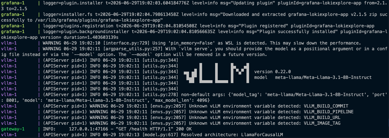
The CUDA graph cache mount
The single most important operational decision in the serving stack is mounting the vLLM compile cache as a Docker volume:
volumes:
  - ~/.cache/vllm:/root/.cache/vllm
Without this, every container restart triggers a full recompilation. With it, vLLM finds the cache, skips compilation, and reaches a healthy state in under two minutes. In a benchmark workflow where you are starting and stopping vLLM repeatedly across variants, this mount is the difference between waiting 90 minutes per run and waiting 2.
The first working request
With the stack running, the first real test is a curl through the gateway:
curl http://localhost:8000/v1/chat/completions \
  -H "X-API-Key: dev-key-change-me" \
  -H "Content-Type: application/json" \
  -d '{
    "model": "meta-llama/Meta-Llama-3.1-8B-Instruct",
    "messages": [{"role": "user", "content": "What is continuous batching?"}],
    "max_tokens": 100
  }'
A response here means every layer is working. The gateway authenticated the key, applied the rate limiter, forwarded the request to vLLM via the singleton AsyncClient, and streamed the response back. Prometheus is already scraping metrics from http://vllm:8001/metrics. Grafana is reading from Prometheus. The dashboard is live.
What “the stack is running” actually means
First, the KV cache prefix cache needs a warm-up pass. The first request through a cold vLLM instance triggers a Triton JIT compilation for a kernel shape it has not seen before. This causes a latency spike that would contaminate the first benchmark results if not accounted for. The benchmark runner sends a silent warm-up request before the timed runs begin.
Second, the GPU needs to be in a stable power state. On the RTX 5090, the first few inference calls after a cold start run at lower clock speeds while the GPU ramps up. Waiting for the healthcheck alone is not enough. The runner waits for the first few requests to complete before it starts recording numbers. When both conditions are met, the stack is ready. Not before.Quantisation Benchmarks
Serving a model in FP16 is the baseline. Every weight is stored as a 16-bit float, nothing is compressed, and you pay the full memory cost. For Llama 3.1 8B, that is roughly 15 GB just for the weights before the KV cache gets any allocation. Quantisation trades some of that precision for smaller weights, faster matrix multiplications, and more room for the KV cache. The question is not whether quantisation helps. It does. The question is how much, and whether the tradeoff is worth it for your workload.
To answer that, inferex runs four variants under identical conditions: FP16, AWQ, GPTQ, and FP8. Same model, same prompts, same concurrency levels, same hardware. The only variable is the quantisation format.
Before running the benchmarks, a quick mental model of what each format actually does.
-
FP16 : Stores every weight as a 16-bit floating point number. Nothing is compressed. The model runs exactly as trained.
-
AWQ (Activation-aware Weight Quantisation): Compresses weights to 4-bit integers, but not uniformly. It observes which weights have the largest effect on activations during a calibration pass, and preserves their precision more carefully than weights that matter less. The insight is that a small fraction of weights are responsible for most of the model’s output quality. Protect those, compress the rest aggressively.
-
GPTQ (Generative Pre-trained Transformer Quantisation): also compresses to 4-bit, but uses a different strategy. It processes the weight matrix one column at a time, finds the optimal quantised value for each weight using an approximation of the inverse Hessian, and compensates for the quantisation error by adjusting the remaining unquantised weights. It is more computationally expensive to quantise than AWQ but produces high-quality 4-bit weights without needing activation data.
-
FP8: Is the simplest of the three. It stores weights as 8-bit floats instead of 16-bit floats, halving the weight memory without changing the numerical representation format. No calibration, no per-weight scaling decisions. The tradeoff is a smaller memory saving than AWQ or GPTQ, but also the smallest risk of quality degradation.
All four run the same model. The only difference is how the weights are stored and how the matrix multiplications happen at inference time.
The benchmark runner design
The runner is built around one principle: variants are data, not code. Each variant is a dictionary with a name, a model path, and any extra flags vLLM needs to serve it. Adding a new variant means adding one entry to a list. The runner logic — starting vLLM, running requests, recording results, stopping vLLM — never changes.
VARIANTS = [
    {"name": "fp16", "model": "meta-llama/Meta-Llama-3.1-8B-Instruct", "extra_args": []},
    {"name": "awq", "model": "/root/.cache/huggingface/hub/Llama-3.1-8B-AWQ", "extra_args": ["--quantization", "awq_marlin", "--dtype", "float16"]},
    {"name": "gptq", "model": "neuralmagic/Meta-Llama-3.1-8B-Instruct-quantized.w4a16", "extra_args": ["--quantization", "gptq"]},
    {"name": "fp8", "model": "meta-llama/Meta-Llama-3.1-8B-Instruct", "extra_args": ["--quantization", "fp8"]},
]
For each variant, the runner spawns a Docker container, polls the health endpoint until vLLM is ready, runs 50 prompts at three concurrency levels (1, 8, 32) using asyncio.gather, records latency and tokens per second for each request, samples VRAM with nvidia-smi, and writes the results to a JSON file. Then it stops the container and moves to the next variant.
The concurrency loop uses asyncio.gather to fire a batch of requests simultaneously. At concurrency 32, all 32 requests are in-flight at the same time. This is what forces vLLM’s continuous batching to work. A sequential loop would never saturate the GPU. It would measure single-request latency, not throughput under load.
Why Docker and not the local vLLM binary
The RTX 5090 is a Blackwell GPU with SM 12.x compute capability. The pip-installed vllm binary does not support it. CUDA 12.9 is required to build kernels for Blackwell, and the standard vLLM pip package ships with an older CUDA toolkit. Attempting to run vllm serve locally produces a device detection failure.
The fix is straightforward: use the official Docker image vllm/vllm-openai:latest , which ships with the correct CUDA toolkit. The runner spawns a container with --gpus all --network host, mounts the HuggingFace and vLLM cache directories, and points it at the model. The container handles the CUDA version requirement. The host only needs Docker and the NVIDIA Container Toolkit.
The four variants
FP16 is the baseline. No quantisation flags, no format conversion, full 16-bit weights. It establishes the throughput and latency floor that every other variant is measured against. AWQ is self-quantised. AutoAWQ compresses the model weights to 4-bit integers using activation-aware scaling. It finds the weights that matter most during inference and preserves their precision. The quantisation is calibrated on 160 samples: 128 from wikitext-2 and 32 domain-specific prompts covering inference engineering topics. The domain prompts matter because calibration data shapes which activations the quantiser treats as important. A model calibrated only on general text may lose precision on the token distributions your actual workload produces.
The AWQ variant requires two extra flags: --quantization awq_marlin and --dtype float16. The awq_marlin flag selects the Marlin kernel backend rather than the standard AWQ kernel. Marlin is a high-performance GEMM kernel optimised for 4-bit weight, 16-bit activation matrix multiplication, which is exactly what AWQ inference does. On modern GPUs it is significantly faster than the default AWQ path. The --dtype float16 flag is required because AWQ does not support bfloat16, which is vLLM’s default.
GPTQ was supposed to be self-quantised too. The plan was to run quantise_gptq.py using auto-gptq. It failed. The installed version of auto-gptq depends on transformers.modeling_utils.no_init_weights, a function that has been removed from recent transformers releases. The alternative, llmcompressor, conflicts with vLLM through a compressed-tensors version clash. Both libraries pin incompatible versions and cannot be installed side by side.
Rather than pin an older transformers release and introduce dependency conflicts across the whole system, the GPTQ variant uses a pre-quantised community checkpoint: neuralmagic/Meta-Llama-3.1-8B-Instruct-quantized.w4a16 from Neural Magic. It is a legitimate 4-bit GPTQ checkpoint of the same model. The tradeoff is calibration data visibility. The AWQ checkpoint was calibrated on known data. The GPTQ checkpoint was calibrated by Neural Magic on data this project has no visibility into.
FP8 is one flag: --quantization fp8. vLLM handles the weight conversion at load time. No separate quantisation step, no calibration data, no community checkpoint. The weights are stored as 8-bit floats rather than 4-bit integers, so the memory saving is smaller than AWQ or GPTQ, but the conversion is lossless enough that no calibration is needed. It is the lowest-friction quantisation option available.
Reading the results
At concurrency 32, the numbers are:
| Variant | Tokens/sec | p95 latency |
|---|---|---|
| FP16 | 87.4 | 2295 ms |
| AWQ | 182.2 | 1115 ms |
| GPTQ | 172.1 | 1155 ms |
| FP8 | 140.0 | 1436 ms |
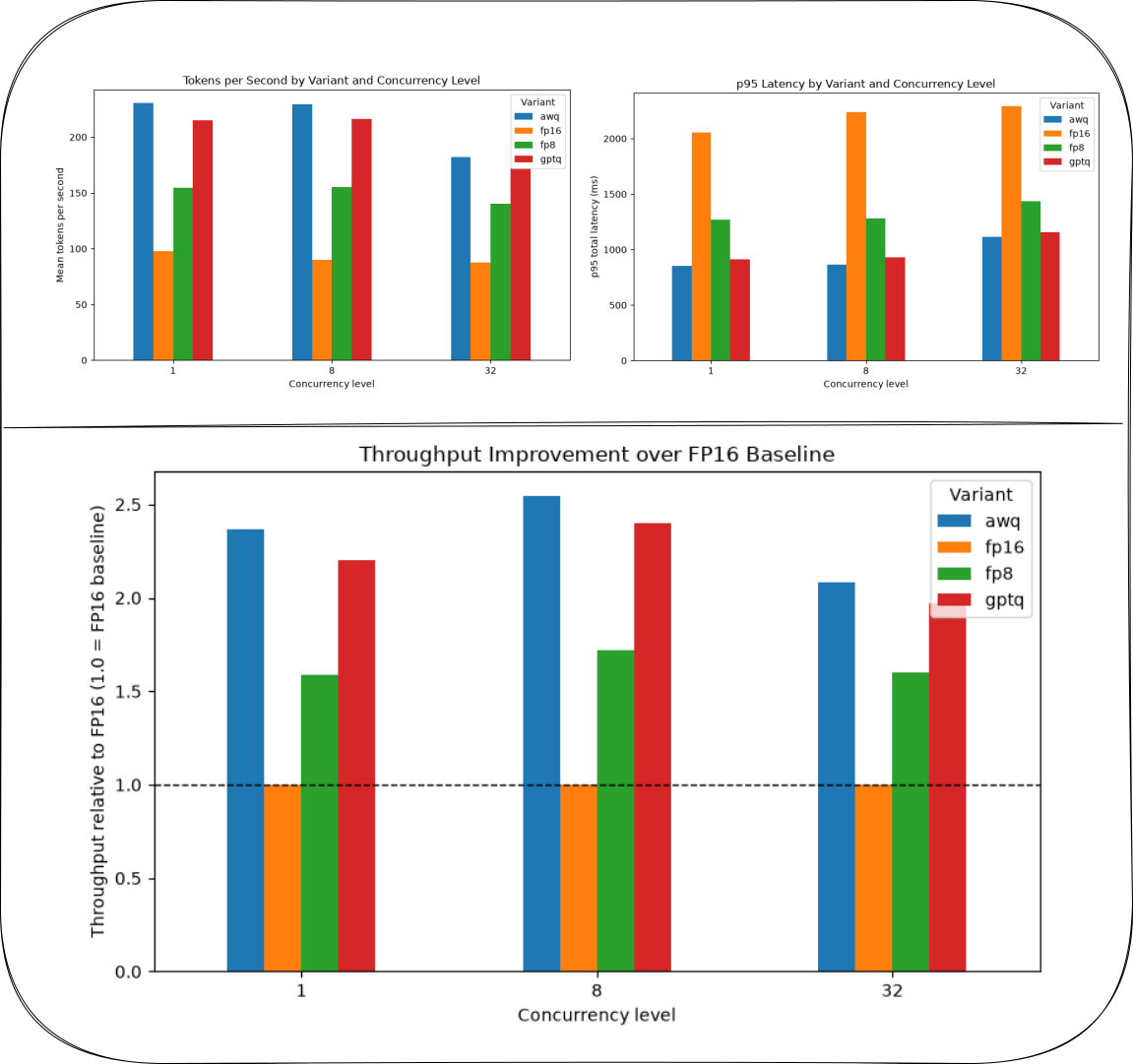
As shown in Figure 5, AWQ delivers 2.1 times the throughput of FP16 at half the p95 latency. That is not a marginal improvement. At production scale, it means serving twice as many users from the same GPU. Where does the speedup actually come from? Not from loading fewer weights. By the time requests are being served, the weights are already in VRAM. The speedup comes from the decode step. Each decode step multiplies the current token's hidden state against every weight matrix in the model. With AWQ, those weight matrices are stored as 4-bit integers and dequantised on the fly using the Marlin kernel. The dequantisation is fast enough that the net operation is faster than doing the full FP16 multiplication, because 4-bit data fits better in the GPU’s cache hierarchy and the memory bandwidth required to load the weights is lower.
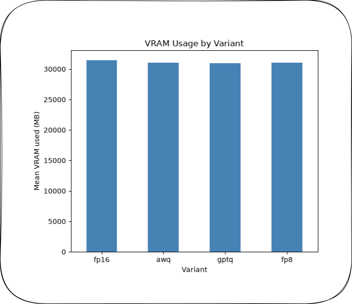
Looking at the VRAM numbers from Figure 6, it tells a confusing story at first. All four variants show approximately 31 GB used, within 482 MB of each other, despite the 4-bit models having roughly a quarter the weight footprint of FP16.
This is not a measurement error. It is how vLLM works.
vLLM’s --gpu-memory-utilization does not size memory to the model. It claims a fixed fraction of total VRAM at startup, 92% in this configuration, regardless of how big the loaded weights are. Whatever is not consumed by weights gets allocated to the KV cache block pool. A smaller model does not reduce vLLM’s total footprint. It grows the KV cache instead.
The real saving from quantisation shows up here:
| Variant | KV cache capacity |
|---|---|
| FP16 | 108,768 tokens |
| AWQ | 183,968 tokens |
| GPTQ | 183,792 tokens |
| FP8 | 158,368 tokens |
AWQ’s smaller weights freed enough VRAM to hold 183,968 tokens in the KV cache versus FP16’s 108,768. That is the difference between supporting roughly 26 simultaneous 4096-token conversations and supporting 44. The saving from quantisation is real. It just does not show up in nvidia-smi. It shows up in how many users you can serve concurrently before the KV cache fills and new requests start queuing.
- For a workload where throughput matters and quality loss is acceptable, AWQ is the clear choice. 2.1 times the throughput at half the latency, with a self-quantised checkpoint calibrated on your own domain data.
- For a workload where you want quantisation with no tooling overhead and no calibration step, FP8 is the pragmatic option. One flag, no separate quantisation run, meaningful throughput improvement over FP16.
- GPTQ sits between the two on throughput but comes with the calibration data caveat. If you use a community checkpoint, you do not know what it was optimised for. For production use where you control the calibration data, GPTQ is worth the tooling effort on a machine where the dependency conflicts do not exist.
- FP16 is the baseline you use when you need to know what the model actually does without any compression in the way. It is not a production choice for cost-sensitive deployments.
Observability with Prometheus and Grafana
A serving stack without observability is a black box. You can tell if it is up or down from the health endpoint, but you cannot tell if it is slow, if the KV cache is filling up, or if one concurrency level is behaving differently from another. Prometheus and Grafana fix that. They are the last two services in the docker-compose stack and they require almost no configuration to be useful.
What vLLM gives you for free
vLLM exposes a /metrics endpoint on the same port as the API. It follows the Prometheus exposition format, which means Prometheus can scrape it directly without any instrumentation code on your side. The metrics vLLM publishes include everything you need to understand serving behaviour: time to first token, generation throughput, request queue depth, KV cache utilisation, and prefix cache hit rate . You do not write a single line of metrics code. You point Prometheus at the endpoint and the data is there.
This is one of the practical advantages of building on a production inference framework rather than rolling your own. The hard observability work is already done.
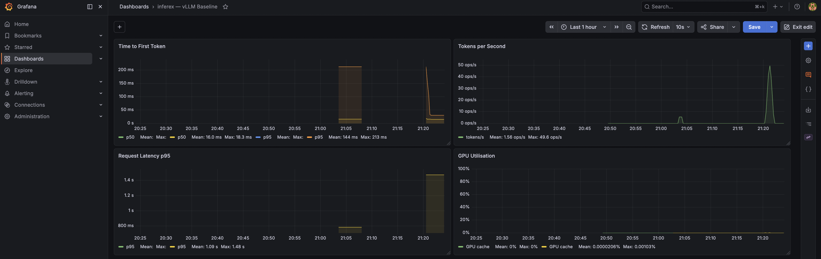
The four dashboard panels
The Grafana dashboard in inferex has four panels, each answering one operational question.
Time to first token (p50 and p95). TTFT is the latency from when the request arrives to when the first token appears in the response. It is the number users feel most directly. p50 tells you what the typical experience is. p95 tells you what the worst 5% of requests experience. The PromQL query pulls from vllm:e2e_request_latency_seconds_bucket and computes the percentile over a 1-minute window.
Generation throughput (tokens per second). This measures how many output tokens vLLM is producing per second across all active requests. It is the primary throughput metric and the one the quantisation benchmarks optimise for. The query uses rate(vllm:generation_tokens_total[1m]).
Request latency p95. End-to-end latency for the full request, from arrival to final token. This is different from TTFT. A request with fast TTFT but slow generation throughput will still show high end-to-end latency. Watching both together tells you whether latency problems are in the prefill phase or the decode phase.
GPU KV cache utilisation. The fraction of KV cache blocks currently in use, expressed as a percentage. When this approaches 100%, new requests start queuing because there is no space to store their attention states. This is the metric that makes the nvidia-smi trap from the quantisation section concrete. The raw VRAM numbers looked similar across variants, but the KV cache utilisation at the same concurrency level tells the real story. The query uses vllm:gpu_cache_usage_perc.
Grafana auto-provisioning
The dashboard is not configured manually. Grafana loads it from a JSON file at startup through its provisioning system. The observability/grafana/provisioning/ directory contains the datasource configuration pointing at Prometheus and the dashboard JSON. When the Grafana container starts, it reads these files and the dashboard is live with no clicks, no imports, no state stored inside the container.
This matters for the same reason the CUDA graph cache mount matters: reproducibility. Anyone who clones the repository and runs docker compose up gets the same dashboard. There is no manual setup step that gets forgotten or done differently on a different machine.
The scrape config change
In the Docker Compose stack, Prometheus scrapes vLLM at vllm:8001. This works because Docker Compose puts all services on the same internal network and resolves service names as hostnames.
When vLLM moves to k3s, this breaks. Prometheus is still running in Docker Compose, but vLLM is now in a k3s pod exposed on a NodePort. The Docker Compose network and the k3s network are separate. vllm:8001 no longer resolves to anything.
The fix is to point Prometheus at the Docker bridge gateway IP instead:
scrape_configs:
  - job_name: "vllm"
    static_configs:
      - targets: ["172.17.0.1:30001"]
172.17.0.1 is the host machine’s address as seen from inside a Docker container. Port 30001 is the k3s NodePort that vLLM is exposed on. From Prometheus’s perspective inside Docker Compose, this address reaches through the Docker bridge network to the host, and from there into k3s. One line change in prometheus.yml is all it takes.
This is the kind of network topology detail that is easy to miss until Prometheus shows a scrape failure and you spend an hour wondering why localhost does not work inside a container.
Docker and Kubernetes
Docker is enough to run inferex. The serving stack works, the benchmarks run, the dashboard is live. So why add Kubernetes at all?
Docker Compose is a single-machine tool . It starts containers, wires them together on a shared network, and stops them. It has no concept of scheduling, no health-based restarts beyond basic container lifecycle, no resource limits that the scheduler enforces, and no way to express that a particular workload requires a GPU. If the vLLM container crashes, Docker Compose restarts it. If the GPU is already in use by something else, Docker Compose has no mechanism to wait for it. If you want to scale to multiple nodes, Docker Compose cannot help you.
Kubernetes adds a scheduling layer. It knows what resources each workload needs, it knows what resources each node has, and it matches them. It enforces resource limits at the scheduler level. It runs health checks and replaces pods that fail them. It provides service discovery through DNS inside the cluster. These are the things a production inference platform actually needs.
Why k3s and not full Kubernetes
Full Kubernetes, installed with kubeadm, requires multiple nodes or a complicated single-node workaround, carries significant control plane overhead, and on a single WSL2 machine competes with the GPU workload for resources. k3s is a certified Kubernetes distribution that runs the same API, accepts the same manifests, and uses the same kubectl commands. Every YAML file written for k3s works unchanged on EKS or GKE. The difference is operational simplicity. k3s installs as a single binary, starts as a systemd service, and is running in under a minute.
For a single-node development cluster on a WSL2 machine, k3s is the right tool . The Kubernetes concepts transfer directly to production. The operational complexity does not.
GPU scheduling: the NVIDIA device plugin
Kubernetes does not know about GPUs out of the box. A pod with resources: limits: nvidia.com/gpu: 1 will sit Pending forever unless the cluster knows how to satisfy that request.
The NVIDIA device plugin is a daemonset that runs on every node with a GPU. It detects the available GPU, advertises it to the Kubernetes scheduler as an allocatable resource (nvidia.com/gpu: 1), and ensures that when a pod is scheduled to use it, the GPU device is correctly passed into the container.
Getting the device plugin working on WSL2 required one extra step: configuring the NVIDIA container runtime for k3s’s containerd. Docker and k3s use different container runtimes. Docker’s GPU support was already working, but k3s runs containerd and needed the NVIDIA runtime configured separately:
sudo nvidia-ctk runtime configure --runtime=containerd
sudo systemctl restart k3s
After that, the scheduler could see the GPU and the device plugin could allocate it to pods.
The WSL2 UVA problem
With the cluster running and the GPU visible, the vLLM deployment was applied and the pod started. It crashed immediately. Not after loading the model. Not during CUDA graph capture. Before loading a single weight.
The logs showed:
RuntimeError: UVA is not available
Tracing the call stack: UvaBuffer.__init__ calls is_uva_available(), which calls is_pin_memory_available(), which calls in_wsl(). The in_wsl() function checks whether the string “microsoft” appears in platform.uname(). On WSL2, it does. So in_wsl() returns True, is_pin_memory_available() returns False, is_uva_available() returns False, and UvaBuffer raises a RuntimeError before the engine core can start.
UVA stands for Unified Virtual Addressing. It is a CUDA mechanism that allows the CPU and GPU to share a single virtual address space, enabling zero-copy memory transfers between them. vLLM’s V2 engine uses a shared memory buffer called UvaBuffer to pass data between the HTTP server process and the engine core process. This requires pinned memory, which requires UVA, which requires /dev/nvidia-uvm. WSL2 does not expose /dev/nvidia-uvm. It exposes /dev/dxg, a DirectX proxy device, instead. Both /dev/nvidia-uvm and /dev/dxg are device nodes used to communicate with NVIDIA GPUs, but they serve fundamentally different environments and driver stacks. CUDA compute works through this path. UVA does not.
The vLLM code was correctly detecting the environment. It was just being more conservative than necessary. On this machine, with this WSL2 kernel version, UVA actually works through the DirectX path. The detection just said it did not.
path = '/usr/local/lib/python3.12/dist-packages/vllm/platforms/interface.py'
with open(path, 'r') as f:
    content = f.read()
old = 'def in_wsl() -> bool:\n    # Reference: https://github.com/microsoft/WSL/issues/4071\n    return "microsoft" in " ".join(platform.uname()).lower()'
new = 'def in_wsl() -> bool:\n    # Patched for WSL2/k3s: disable WSL detection to enable UVA\n    return False'
content = content.replace(old, new)
with open(path, 'w') as f:
    f.write(content)
Dockerfile.vllm extends the official vLLM image and runs this script at build time:
FROM vllm/vllm-openai:latest
COPY patch_vllm.py /tmp/patch_vllm.py
RUN python3 /tmp/patch_vllm.py
The result is inferex-vllm:latest, a patched image that behaves identically to the upstream image on native Linux but does not disable UVA on WSL2. The patch is baked into the image, travels with it through k3s ctr images import, and survives container restarts.
The assert inside patch_vllm.py is intentional. If a future upstream vLLM update changes the in_wsl() function signature, the assert fires and the build fails visibly rather than silently applying a partial patch.
Belt-and-suspenders: VLLM_ENABLE_V1_MULTIPROCESSING
The pod spec also sets VLLM_ENABLE_V1_MULTIPROCESSING: "0". This disables the multiprocessing engine mode that requires UVA, as a fallback. If the image patch ever fails on an update, this environment variable engages the single-process path rather than crashing. Either fix alone is sufficient. Together they cover the failure mode where the upstream image changes faster than the patch is rebuilt.
The LimitRange incident
After getting the vLLM pod running, the gateway pod might not schedule just as this event log shown below:
0/1 nodes are available: 1 Insufficient nvidia.com/gpu
The gateway does not use a GPU. It is a FastAPI process. It has no GPU resource request in its deployment manifest.
The problem was a LimitRange object applied to the inferex namespace. A LimitRange sets default resource requests and limits for every container in a namespace that does not specify its own. The GPU LimitRange was defaulting every container to nvidia.com/gpu: 1. The gateway pod inherited this default, the scheduler saw it needed a GPU, and since the GPU was already allocated to vLLM, the gateway pod could not be scheduled.
The fix was to delete the LimitRange from the cluster. The manifest is kept in k8s/gpu-resource-limits.yaml for reference but is not applied. The key takeaway here is that namespace-scoped defaults apply to everything in the namespace with no selector mechanism. On a single-GPU node, a GPU LimitRange effectively blocks any CPU-only workload from running alongside the GPU workload.
Hybrid architecture
vLLM and the gateway run as k3s pods. Prometheus and Grafana stay in Docker Compose. The GPU-scheduled workloads belong in Kubernetes where the scheduler can manage them properly. The observability stack has no GPU requirement and no reason to carry the complexity of k3s GPU scheduling. Keeping them in Docker Compose means one less set of manifests to maintain and one less failure mode to debug.
The cost of this split is one network boundary. Prometheus cannot reach the k3s vLLM pod using the Docker Compose service name vllm:8001 because the two stacks are on separate networks. The solution is to point Prometheus at the Docker bridge gateway IP, 172.17.0.1, and the k3s NodePort 30001. From inside a Docker container, 172.17.0.1 is the address of the host machine. Port 30001 is where k3s exposes the vLLM service externally. One line in prometheus.yml is the entire cost of the hybrid architecture.
The HPA manifest
k8s/hpa.yaml defines a HorizontalPodAutoscaler targeting the vLLM deployment. It scales between 1 and 4 replicas based on CPU utilisation. It is not applied to the cluster.
A single-GPU node cannot schedule a second vLLM replica. There is only one GPU and each vLLM pod requests it exclusively. Applying the HPA would cause it to attempt scaling, fail to schedule additional pods, and generate a stream of Insufficient nvidia.com/gpu events.
On a multi-GPU node or a multi-node cluster, this is exactly how you would autoscale an inference deployment. It documents the intended production behaviour.
vLLM and SGLang Engine Comparison
While vLLM was established as the baseline in the earlier stage. This section asks a different question: is vLLM actually the best engine for this workload, or is there something better?
SGLang is the main alternative worth benchmarking. It was built by the same research community that produced FlashAttention and PagedAttention , and it makes a specific architectural claim: its KV cache management strategy, RadixAttention , is more efficient than vLLM’s PagedAttention for workloads with shared prefixes. At high concurrency with repeated prompt patterns, SGLang should win.
It did not. Here is why.
RadixAttention vs PagedAttention
vLLM’s PagedAttention divides the KV cache into fixed-size page blocks, similar to how an operating system manages virtual memory. Each request gets pages allocated to it as it generates tokens. When the request finishes, the pages are freed. There is no sharing between requests. If two requests have identical system prompts, both requests compute and store the KV values for that system prompt independently.
SGLang’s RadixAttention stores the KV cache as a tree of shared prefixes. If two requests share a common prefix, the KV values for that prefix are computed once and reused by both. The tree uses LRU eviction to manage capacity. For workloads where many requests share a system prompt or few-shot examples, RadixAttention avoids redundant prefill computation entirely.
For the inferex benchmark, which runs 50 fixed prompts in repeated batches, RadixAttention should have a meaningful advantage. By the time concurrency level 8 begins, many of the prompt prefixes are already cached from concurrency level 1.
The overlap scheduler
RadixAttention is one half of SGLang’s performance story. The overlap scheduler is the other half, and it is the more important one for throughput at high concurrency.
vLLM’s continuous batching works in discrete steps. The GPU runs a forward pass, the CPU processes the results, the CPU decides what goes in the next batch, and then the GPU runs the next forward pass. During the CPU scheduling window, the GPU is idle.
SGLang’s overlap scheduler pipelines these two phases. While the GPU is running the current forward pass, the CPU is already preparing the next batch. By the time the GPU finishes, the next batch is ready. The GPU never idles waiting for a scheduling decision. At high concurrency, where scheduling decisions happen frequently and the GPU is the bottleneck, this overlap is where SGLang’s throughput advantage over vLLM comes from.
Running the comparison
The quantisation benchmark runner in benchmarks/runner.py was designed for vLLM variants. SGLang uses a different Docker image, a different launch command, and a different port. Rather than modify the existing runner, a new file benchmarks/runner_engine_compare.py was created.
The two runners share the request logic. run_single, run_concurrency_level, and get_vram_mb are imported directly from runner.py. The new file adds start_vllm_engine and start_sglang_engine as separate functions, each hardcoding the launch command for its engine. An ENGINES list drives the orchestration, the same variant-as-data pattern from ealier stage:
ENGINES = [
    {
        "name": "vllm",
        "base_url": "http://localhost:8001",
        "result_file": "vllm.json",
        "start_fn": start_vllm_engine,
    },
    {
        "name": "sglang",
        "base_url": "http://localhost:8002",
        "result_file": "sglang.json",
        "start_fn": start_sglang_engine,
    },
]
The SGLang launch command runs on port 8002 so both engines could theoretically run simultaneously in future. For this benchmark they run sequentially, one after the other, to avoid GPU contention.
The first SGLang run crashed at request 40 of 50 during concurrency level 1:
torch.AcceleratorError: CUDA error: unknown error
The traceback led to copy_done.synchronize() inside the overlap scheduler. The same class of failure as the vLLM UVA crash in phase 3: a CUDA synchronisation primitive that requires /dev/nvidia-uvm, which WSL2 does not expose. Adding --disable-overlap-schedule to the SGLang launch command stabilised it. The benchmark completed cleanly on the second run.
The counter-intuitive result: vLLM won
At concurrency 32, the numbers are:

vLLM was faster on every concurrency level. SGLang was slower on throughput and worse on tail latency.
What the logs actually showed
RadixAttention was working. The SGLang logs showed prefix cache hits accumulating across requests. By concurrency level 8, the cached token count was over 600 tokens per request. The tree cache was doing exactly what it is supposed to do.
Prefill batch, #new-seq: 7, #new-token: 7, #cached-token: 609
Seven new sequences, seven new tokens to prefill, 609 tokens served from the cache. That is a very high cache hit rate. SGLang was not losing because of RadixAttention.
Why it still lost
SGLang lost because --disable-overlap-schedule removed the one mechanism responsible for its throughput advantage at high concurrency. RadixAttention reduces prefill work. The overlap scheduler is what converts that reduced work into higher GPU utilisation. Without the scheduler pipeline, the GPU idles during every scheduling window, and vLLM’s more mature continuous batching implementation fills that idle time better.
The result is accurate but not representative of what SGLang actually does on production hardware . The benchmark measured SGLang without its primary throughput mechanism, then compared it to vLLM with everything enabled. Under those conditions, vLLM winning is expected.
What the result would look like on native Linux
On a native Linux node, /dev/nvidia-uvm is available. The overlap scheduler runs without modification. SGLang’s architecture is designed to win at high concurrency, and on native Linux at concurrency 32 with a shared-prefix workload, the expected result is that SGLang outperforms vLLM. The RadixAttention cache hit rate seen in these logs would be the same. The overlap scheduler would keep the GPU busy during scheduling windows that vLLM leaves idle. Both advantages would be active simultaneously.
The benchmarks in this project cannot confirm that claim. But the architecture explains it, and the logs show that one half of SGLang’s advantage was fully active even on WSL2.
The nvidia-smi sentinel value
During the SGLang run, get_vram_mb() returned 17592181910845 for every concurrency level. Not a real VRAM reading. 17592181910845 is 0xFFFFFFFFFFFF in hexadecimal, a sentinel overflow value that nvidia-smi returns when it cannot read the GPU memory counter correctly. The subprocess call succeeded, the output parsed as an integer, and the corruption was invisible until the number was compared against a known physical maximum.
The fix is a threshold check in get_vram_mb():
def get_vram_mb() -> int | None:
    result = subprocess.run(
        ["nvidia-smi", "--query-gpu=memory.used", "--format=csv,noheader,nounits"],
        capture_output=True, text=True, timeout=10,
    )
    try:
        value = int(result.stdout.strip().splitlines()[0])
        if value > 40_000:
            return None
        return value
    except (ValueError, IndexError):
        return None
The RTX 5090 has 32 GB of VRAM. Any reading above 40,000 MB is not a real value. Return None instead and let the caller handle the absence of data rather than silently recording garbage.
The VRAM readings for the engine comparison are all None as a result. For this particular comparison it does not matter. Both engines load the same FP16 model. The VRAM footprint is identical. The interesting comparison is throughput and latency, and those numbers are clean.
Conclusion
Building inferex produced results that reading documentation could not. Documentation describes how systems are supposed to work. Running them under load, on real hardware, with real constraints, reveals how they actually work.
1. The nvidia-smi trap. Every quantisation variant showed approximately 31 GB VRAM used, despite 4-bit models having a quarter of FP16's weight footprint. The saving from quantisation does not appear in memory readings. It appears in KV cache capacity, AWQ expanded the cache from 108,768 to 183,968 tokens on the same hardware budget. Without running the benchmark, that distinction is easy to miss. With it, it becomes the central insight for any production quantisation decision.
2. WSL2 and the kernel boundary. The same constraint surfaced twice in different code paths. vLLM's in_wsl() detection disabled UVA before the engine could start. SGLang's overlap scheduler hit copy_done.synchronize() and crashed for the same underlying reason, both require /dev/nvidia-uvm, which WSL2 does not expose. Two different engines, two different failure modes, one root cause. That pattern is only visible when you run the engines rather than read about them.
3. The counter-intuitive benchmark result. SGLang was expected to win at high concurrency. It did not. RadixAttention was working, the logs confirmed 600+ cached tokens per request, but the overlap scheduler, disabled to stabilise the run, was the mechanism that would have converted those cache hits into higher throughput. The result is accurate but not representative. Knowing the difference between those two things is what benchmark-driven development gives you.
The question every component had to answer was: does this reflect how a production inference platform is actually built? After running four quantisation variants, two inference engines, a Kubernetes deployment, and a full observability stack on consumer hardware, the answer is closer to yes than it was at the start.